From survey items to a scale, then on to regression and QCA: a step-by-step guide
How to define a multi-item concept such as brand trust from theory, examine it with factor analysis and alpha, build subscales, and use them in regression and QCA, with an example in R.
marketing
tutorial
Author
Yuki Toyoda
Published
October 8, 2026
NoteHow this article, the app, and the R script fit together
The step-by-step articles on this blog come with an app (a tool that runs in your browser) that lets you try the same procedure. The three have different roles:
The article explains the ideas and the procedure. The calculations are shown as R code.
The app (Scale Maker) reads your data (CSV) and shows the same calculations as the article on screen. You can learn the flow of the procedure and the meaning of the numbers without using R.
The R script: the app can produce an R script that reproduces the results of your settings on screen. You can run it in R and confirm that the numbers match the app. In research, you can also keep the script as a record of your analysis.
If you use R, start from the code in the article. If you learn with the app, read the article while looking at the numbers in the app first, and then reproduce them with the R script when you are comfortable.
The question this article answers
Research in marketing and management deals with concepts such as brand trust, perceived quality, customer satisfaction, and price sensitivity, which are hard to measure with a single question. These concepts are called constructs, and we measure them with several questionnaire items.
Suppose we measure brand trust with these three items:
Q1: This brand is sincere
Q2: I think this brand keeps its promises
Q3: I feel secure using this brand
What we want to know is not the effect of Q1, Q2, or Q3 separately. We want to know how brand trust, the three items taken together, relates to outcomes such as purchase intention. We also often want to use such constructs in later analyses: regression, logistic regression, QCA, cluster analysis, decision trees, and so on.
Structural equation modeling (SEM) is a wonderful method, but you do not have to start with it (and if you use it without understanding its characteristics, it can do more harm than good). What matters is not which method is more advanced, but how you measure the constructs of your research, and how you analyze them in the way that best fits your research question.
This article presents a procedure that works well for MBA research and empirical studies, with an example in R. The example data are generated with random numbers (they are not real survey data).
Scope of this article
We deal with constructs that you define in advance from theory and measure with several items. This does not deny the value of exploratory studies that look for constructs in the data.
We deal with measurement like brand trust, where we assume that one underlying construct drives the answers to several items in common. A person with high brand trust answers high on Q1, Q2, and Q3 alike. Therefore, the items are expected to correlate with one another (this kind of measurement is called reflective measurement).
A different case is building a “customer behavior index” by combining purchase frequency, purchase amount, and years of use. A person who buys often does not necessarily spend a lot. The items need not correlate strongly, so the factor analysis and alpha procedure shown here does not apply as it is. It is not true that “for any index, you can raise alpha and take the average.”
The overall flow
Define the construct from theory and prior research
Prepare several questionnaire items for each construct
Use exploratory factor analysis (EFA) to examine, in an exploratory way, whether the item groupings you expected are consistent with the data
Align the direction of reverse-keyed items
Check internal consistency (Cronbach’s alpha)
Build subscales by averaging items
Use the subscales in regression and QCA
Let us go through them in order.
TipFor readers who learn with the app (this article)
“Example 3” in the app (Scale Maker) uses the same data as this article. Steps 2 to 7 in the app correspond to steps 3 to 6 in this article. Regression and QCA are done in R. The app’s calculation is the same as R’s standard promax. Depending on the version of psych, the third decimal place of the factor loadings can differ slightly.
Step 1: Define the construct from theory (before factor analysis)
This is the most important step. Before factor analysis, the researcher has to decide what to measure. Concepts such as “brand trust” and “perceived quality” are not things that statistical software finds for you automatically.
The approach to avoid looks like this:
“Let’s ask 20 questions for now, run a factor analysis, and name the factors that come out.”
This is a misunderstanding that beginners especially tend to fall into. The preferred order is as follows.
From prior research and theory, define what brand trust is, and think about the questionnaire items needed to observe it. When you prepared Q1 to Q3 above, you already held a theoretical expectation before the survey began: “these three items should be measuring one construct, brand trust.” You then run a factor analysis to check whether these three items actually move in the same direction in the real response data.
We do not build theory from factor analysis; we examine, in an exploratory way, whether the data are consistent with a measurement structure that we assumed from theory. This is why research on prior studies and theory beforehand is so important.
Factor analysis is not a machine that sorts items automatically
Suppose you run a factor analysis on 20 items and get four factors. That alone does not let you say that “human attitudes consist of four constructs.” What factor analysis shows is only the statistical fact that “in this sample, the correlation structure of this item set can be summarized fairly well by about four common factors.”
Whether those four factors are brand trust, quality evaluation, or brand attachment is not decided by the statistical result. You have to interpret them using prior research, the content of the items, the definition of the construct, and the purpose of the research. Please avoid giving plausible-sounding names to whatever factors come out.
Statistical grouping and theoretical validity are different things
Suppose four items, “high quality,” “good design,” “reasonably priced,” and “a well-known brand,” group into one factor statistically. That alone does not mean you may call the factor “brand value.” There are several possible reasons why items group statistically:
They really measure the same construct
Respondents tend to rate everything high
There is a halo effect
The item wordings are similar
There is a method effect from the same response format
A high factor loading does not prove that the items belong to the same concept in theory.
Step 2: Prepare several items for each construct
As a rule, prepare several items for each construct. Do not line up items that merely rephrase the same sentence. Items with the same meaning tend to raise Cronbach’s alpha, but this does not mean that the construct is covered adequately. It is desirable for the items to represent different aspects of the construct appropriately.
For example, compare these two ways of measuring brand trust.
An example of rephrasing
This brand is trustworthy
This brand is reliable
This brand is dependable
All three ask almost the same thing. The answers will be similar, so alpha will be high. But if you duplicate content to raise alpha, you can no longer tell whether the necessary aspects of brand trust are covered. Whether they are covered has to be examined separately. Note that when the concept you want to measure is narrow, items with close meanings can be appropriate, and they can also help average out errors caused by differences in wording.
An example of different aspects
I think this brand keeps its promises (the aspect of fulfilling promises)
This brand is sincere (the aspect of caring about the other party)
I feel secure using this brand (the aspect of reassurance in use)
All three are part of “brand trust,” but each looks at a different aspect, so the concept is captured more broadly. However, if you vary the aspects too much, the correlations among items fall and the items no longer form one factor. In light of the definition of the construct, choose items within the range where you can say they are “different aspects of the same concept.”
TipA questionnaire tip: labeling the options of a 7-point scale
There are two main ways to label the options.
Put a verbal label on all seven options: the meaning of each option is clear. On the other hand, words such as “very,” “extremely,” and “quite” feel different in strength to different people.
Label only the two ends and leave only numbers in between: this makes it easier to avoid differences in how strongly the words are felt.
Disagree 1 - 2 - 3 - 4 - 5 - 6 - 7 Agree
Which one to use depends on the purpose of the research and on the format of the existing scale you use. What deserves attention is that, in either form, treating the scores as equally spaced numbers is the analyst’s assumption (a simplification). The way of labeling does not guarantee equal spacing. In this article, we treat responses as numbers under this assumption.
If a scale has been used widely in prior research, using the existing scale is often better than writing items from scratch, because its validity has been examined and it is easy to compare with other studies. This does not mean, however, that “the existing study used three items, so we can use them as they are.” If the industry, culture, respondents, or purpose of the survey differ, the same factor structure may not be reproduced. Even with an existing scale, it is worth checking the structure in your own data.
Example data
From here we follow the steps in R. Suppose we measured nine items on a 7-point scale. The theoretical expectation is the following three constructs.
Construct
Item
Wording (example)
Brand trust
Q1
This brand is sincere
Q2
I think this brand keeps its promises
Q3
I feel secure using this brand
Perceived quality
Q4
This brand’s products are of high quality
Q5
This brand’s products perform well
Q6 (reverse-keyed)
The quality of this brand’s products varies
Price sensitivity
Q7
I notice even small price differences
Q8
I am tempted to buy when there is a discount
Q9
If products are similar, I choose the cheaper one
The wordings are examples (the data are generated with random numbers, and no actual survey corresponds to these wordings).
The outcome variable Y is purchase intention (one item on a 7-point scale).
Note
In this article, we treat 7-point responses as numbers and use Pearson correlation and linear regression. This is a common simplification in practice. If the response distributions are strongly skewed, you can also consider treating them as ordinal. For example, in factor analysis you can use polychoric correlations (fa(..., cor = "poly")). If purchase intention is measured with a single item, you can choose ordinal logistic regression instead of linear regression.
The following code creates the example data (the random seed is fixed, so you get the same data).
set.seed(2026)n <-300Phi <-matrix(c(1.0, 0.5, -0.2,0.5, 1.0, -0.1,-0.2,-0.1, 1.0), 3, 3, byrow =TRUE) # correlations among the 3 constructsFm <-matrix(rnorm(n *3), n) %*%chol(Phi)lam <-c(.80,.75,.70, .78,.72,.68, .75,.70,.65) # item loadings (the "true" values)fac <-rep(1:3, each =3)to7 <-function(z) as.integer(cut(z, c(-Inf,-1.6,-1.0,-0.4,0.4,1.0,1.6,Inf))) # make 7-point responsesX <-sapply(1:9, function(j) to7(lam[j] * Fm[, fac[j]] +sqrt(1- lam[j]^2) *rnorm(n)))X[, 6] <-8L - X[, 6] # record Q6 as a reverse-keyed itemcolnames(X) <-paste0("Q", 1:9)b <-c(.45, .30, -.20) # effects of the 3 constructs on purchase intentionv <-drop(t(b) %*% Phi %*% b) # variance of the signal part (including correlations among the constructs)Y <-to7(drop(Fm %*% b) +sqrt(1- v) *rnorm(n)) # add error so that the total variance is 1dat <-data.frame(X, Y = Y)head(dat)
Step 3: Examine how the items group, with exploratory factor analysis
Once the items are ready, examine how they group by using exploratory factor analysis (EFA). The role we expect of EFA here is not “to invent constructs from a state of knowing nothing.” It is to examine, in an exploratory way, whether the item structure we assumed from theory is consistent with the actual data. EFA is different from confirmatory factor analysis (CFA), which specifies in advance as a model which item measures which factor and tests it. The result of EFA is material for judging consistency with your expectation; it does not mean that the measurement structure has been verified.
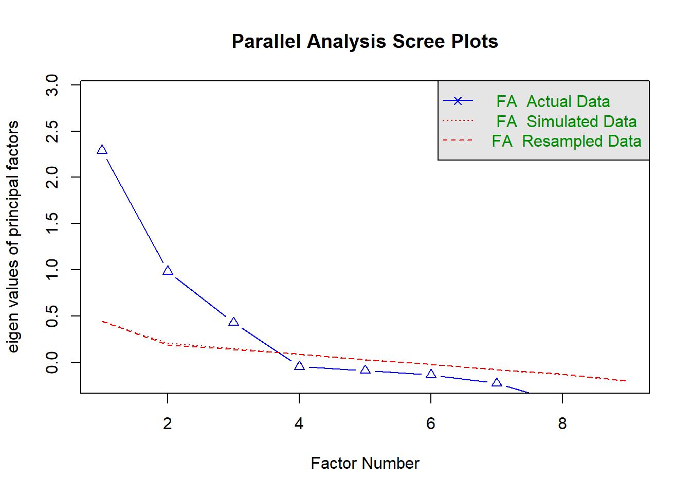
First, as a guide to the number of factors, look at the eigenvalues of the correlation matrix and at parallel analysis. The count of eigenvalues of 1 or more is only a rough guide. Parallel analysis compares the eigenvalues of the real data with those obtained from random data, and uses the comparison as a clue to the number of factors. Decide the number of factors together with your theoretical expectation. Then extract three factors by principal axis factoring with promax rotation.
To make the results easy to reproduce, this article uses rotate = "Promax" (with a capital P). The lowercase "promax" is not wrong, but its internal normalization differs, so the values change slightly.
min.err = 1e-8, max.iter = 1000 makes the iterations of principal axis factoring converge under strict criteria. The default criteria are loose, so the extraction can differ slightly around the third decimal place. To make the results match, this article uses the strict criteria.
Note also that the promax rotation calculation differs a little between versions of psych, and the third decimal place of the loadings can change (we confirmed a difference of at most 0.003 between psych 2.4.1 and 2.6.5). The extraction (principal axis factoring) gives the same result. The interpretation does not change.
Here is what to look at.
Number of factors: Look at the eigenvalues (the number of those at 1 or more) and the parallel analysis figure (the number of factors whose real-data eigenvalues exceed those from random data), and check whether they are consistent with the three factors we expected from theory.
Item groupings: Check whether Q1 to Q3, Q4 to Q6, and Q7 to Q9 load on the same factor, as expected. (Labels such as PA1 only indicate the order. Read the meaning of a factor from the items that load on it.)
The negative loading of Q6: Q6 has the opposite sign to Q4 and Q5 within the same factor. This is a clue that Q6 may be a reverse-keyed item. However, the sign is only a guide (the sign of a whole factor can be flipped). Whether an item is reverse-keyed is decided by the meaning of the wording.
Whether any item loads strongly on several factors (cross-loading).
For example, if only Q3 loaded strongly on the perceived quality factor, consider the following before deleting it:
Was the wording of Q3 appropriate?
Are brand trust and perceived quality conceptually too close?
Is there a problem with the translation or the phrasing?
Did respondents read it with a meaning different from the one we expected?
Use the result of EFA not as a “keep or delete verdict,” but as material for understanding the gap between the measurement model assumed from theory and the actual response behavior. If you mechanically delete a content-wise important item only because its loading is a little low, you may damage content validity.
Step 4: Align the direction of reverse-keyed items
Q6 is a reverse-keyed item. In practice, it is easier to follow if you decide the reverse-keyed items from the meaning of the wording before the analysis and align their direction in advance. In this article, we ran the EFA first, to show that a negative loading can be a clue. Use the minimum and maximum of the scale (here 1 and 7) and compute (minimum + maximum) − original value, that is, 8 - Q6. For 1 to 7, use 8 - Q6; for 1 to 5, use 6 - Q6. The same formula also works for a scale whose minimum is not 1 (for example, 0 to 10). Use the ends of the scale on the questionnaire (1 and 7 for a 7-point scale), not the minimum and maximum observed in the data. Whether an item is reverse-keyed is decided by the meaning of the wording (theory).
Once you have examined the factor structure, check the internal consistency of each item group. A typical index is Cronbach’s alpha. For example, \(\alpha = .84\) indicates that the item group has relatively high internal consistency.
A high alpha does not prove a one-factor structure. Alpha is an index of internal consistency, not an index for verifying factor structure. Also, alpha alone cannot tell you about reliability in general or about validity. The order is: examine the structure by factor analysis, then check the internal consistency of that item group.
Alpha tends to rise as the number of items grows. If needed, you may use McDonald’s omega alongside it.
Step 6: Build the subscales
Once you have examined the structure and checked the internal consistency, build a subscale for each construct. Usually the simple mean of the items is the default.
A scale built from a simple mean still contains measurement error. An ordinary regression that uses such a scale does not model the measurement error explicitly. Therefore, the coefficients you obtain are not necessarily the same as the relationships among the latent constructs themselves. With low reliability, this effect can be larger. In multiple regression especially, the effect of measurement error also depends on the correlations among the predictors, so you cannot judge the effect on the coefficients from reliability alone.
A simple mean has the following advantages:
The calculation is clear and highly reproducible
It depends relatively little on the sample
The unit of the original response scale is kept, so it is easy to interpret
It can be used in both regression and QCA
Why not use factor scores?
Using factor scores is not wrong in itself. However, factor scores have problems: the weights depend on the sample, the values change with the estimation method, the meaning of the score itself is hard to grasp, and the scale may not be the same in another sample. Unless there is a special reason, a policy of using simple-mean scales whose reliability has been checked is quite reasonable for MBA-level research.
Where does confirmatory factor analysis (CFA) come in?
In exploratory MBA research, it is practical to build simple-mean scales based on the content of the items, the EFA results, and internal consistency. However, that alone does not mean that the validity of the measurement has been fully established.
How far to verify depends on the track record of verification of an existing scale, the extent of your changes, and the strength of the claim the research needs to make. When you want to verify the measurement structure explicitly, or when you have built a new scale or changed one substantially, consider additional verification such as CFA. In CFA, you specify in advance, as a model, which item measures which factor. If an existing measurement model is clear, you can also start with CFA without going through EFA. So there is no fixed order of “always do CFA after EFA.”
If your sample is large enough, a better approach is to split the sample, running EFA on one part for exploration and CFA on the other for verification. Even if you do run CFA, you do not necessarily have to use the CFA factor scores afterward.
Step 7: Use the subscales in regression and QCA
Regression
Once you have the subscales, you can run an ordinary regression.
summary(lm(Y ~ Trust + Quality + Price, data = dat))
Call:
lm(formula = Y ~ Trust + Quality + Price, data = dat)

Residuals:
     Min       1Q   Median       3Q      Max
-3.11817 -0.87767  0.06223  0.76259  2.85718

Coefficients:
            Estimate Std. Error t value Pr(>|t|)
(Intercept)  1.42862    0.37338   3.826 0.000159 ***
Trust        0.57160    0.06622   8.632 3.78e-16 ***
Quality      0.36507    0.05991   6.093 3.44e-09 ***
Price       -0.27133    0.05812  -4.668 4.61e-06 ***
---
Signif. codes:  0 '***' 0.001 '**' 0.01 '*' 0.05 '.' 0.1 ' ' 1

Residual standard error: 1.157 on 296 degrees of freedom
Multiple R-squared:  0.4399,    Adjusted R-squared:  0.4342
F-statistic: 77.49 on 3 and 296 DF,  p-value: < 2.2e-16
QCA
QCA needs a value of each condition for each case. In this example, the subscales of brand trust, perceived quality, and price sensitivity can be used as conditions. In fuzzy-set QCA (fsQCA), you calibrate each of them into set membership (values from 0 to 1). The outcome, purchase intention Y, is also calibrated into the set “high purchase intention.”
Then, for example, for the combination “high brand trust, high perceived quality, and low price sensitivity,” we examine a sufficiency relation such as the following (~ is negation and * is logical AND).
This expression is not an analysis result. It is an example of a combination to examine.
Decide the calibration anchors (full membership, full non-membership, and the crossover point) from the meaning of the set, not by mechanically converting the scale mean to a 0 to 1 range.
Y in the example measures purchase “intention.” Please write it separately from actual purchase “behavior.”
If you run regression and QCA on the same subscales, you can look at the same phenomenon from different viewpoints. Regression looks at the average association when the other variables are held constant. QCA looks at which combinations of conditions lead to the outcome. The two are better seen as complementary methods with different viewpoints than as competing methods. If you use common subscales, the measurement is unified across the two analyses.
What to report
In a paper or report, writing at least the following lets readers follow your procedure:
The definition of each construct and the source of the items (an existing scale, or one you created)
The sample size and how missing values were handled (for example, only complete cases were used)
The estimation method of the factor analysis (such as principal axis factoring), the rotation (promax), and the basis for the number of factors
The reverse-keyed items
The number of items and the alpha of each subscale
How the subscales were built (the simple mean of the items)
The whole procedure in a few words
A standard practical procedure has the following 11 stages. Steps 1 to 7 of this article rearrange these stages, except CFA (8) and SEM (11), in the order of building a scale (with a check of reverse-keyed items added).
Define the construct from prior research
Prepare several questionnaire items for each construct
Hold in advance a theoretical expectation of “which item measures which construct”
Use EFA to examine, in an exploratory way, whether that expectation is consistent with the actual data structure
Examine the items from both theoretical and statistical viewpoints
Check internal consistency with Cronbach’s alpha (and McDonald’s omega if needed)
Build subscales by simple means
Verify the measurement structure further with CFA, if needed
Use the subscales in regression and similar analyses
In QCA, calibrate the subscales and use them
If the structure among latent variables is itself the research aim, consider SEM
The most important point is not “collect data and then look for meaning by factor analysis,” but “define the meaning from theory, and use factor analysis to examine, in an exploratory way, whether that meaning also holds in the data.”
\[
\text{theory} \rightarrow \text{construct} \rightarrow \text{items} \rightarrow \text{examination of the measurement structure} \rightarrow \text{scaling} \rightarrow \text{hypothesis tests by regression, QCA, etc.}
\]
You do not need to decide mechanically that “we use constructs, so we use SEM.” What matters is that the research question, the theory, the measurement, the way of building scales, and the method of analysis are consistent with one another.
This article does not cover why you might not use SEM, or how SEM compares. I plan to write about that in a separate article (Notes).
What to read next
The subscales you built in this article can also be used in QCA. While regression looks at the average association when the other variables are held constant, QCA looks for which combinations of conditions lead to the outcome. ThSQCA is an R package that shows how those combinations change when you move the target level (the threshold) of the outcome.
The results were checked in the following environment. A fixed seed produces the same data, but results can change slightly with different versions of R or of the packages.