ThSQCA for beginners, part 1: your first threshold sweep

This is the first part of a beginner’s series on ThSQCA, an R package for threshold-sweep qualitative comparative analysis (QCA). You do not need to know QCA beforehand. By the end of this post you will have run a threshold sweep yourself and read its result.

The one idea you need

QCA looks for combinations of conditions that are sufficient for an outcome. Suppose we study customer loyalty. A combination such as “high quality AND high service” is sufficient for high loyalty if (almost) every customer who has both also has high loyalty.

To do this, QCA first has to decide who counts as “high”. With survey scores from 0 to 10, we pick a threshold: a customer is “high” on a variable when the score is greater than or equal to the threshold. In this series, each score is split at the threshold into “high” and “not high” (crisp-set QCA).

Here is the catch. A threshold of 7 and a threshold of 8 are both reasonable, but they can lead to different answers. A normal QCA analysis picks one threshold and reports one answer. ThSQCA reruns the same analysis for a whole range of thresholds and puts all the answers in one table, so you can see where the answer holds and where it changes.

ThSQCA does not replace the QCA package. For every threshold, it calls QCA’s truthTable() and minimize() for you, with identical settings each time, and collects the results.

Step 1: install the packages

Run this once. (If you already installed them, skip it.)

install.packages(c("QCA", "ThSQCA"))

Then load ThSQCA in every new R session:

library(ThSQCA)

Step 2: create a small practice data set

To keep things reproducible, we simulate 400 customers. Each has four scores from 0 to 10: loyalty (LOY), and evaluations of quality (QUA), service (SER), and store environment (ENV). In this simulated world, loyalty is high when quality and service are both high, or (a little less strongly) when quality and environment are both high. A good analysis should discover this.

make_demo_data <- function(n = 400, seed = 2026) {
  set.seed(seed)
  clip <- function(x) pmin(10, pmax(0, round(x)))
  QUA <- clip(rnorm(n, 6, 2))
  SER <- clip(rnorm(n, 6, 2))
  ENV <- clip(rnorm(n, 6, 2))
  core <- pmax(pmin(QUA, SER), pmin(QUA, ENV) - 1)
  LOY  <- clip(core + rnorm(n, 0, 0.7))
  data.frame(LOY, QUA, SER, ENV)
}

demo <- make_demo_data()
head(demo)

  LOY QUA SER ENV
1   7   7   9   3
2   5   4   7   5
3   4   6   4   4
4   6   6   6   4
5   5   5   4   7
6   0   1   2   5

Each row is one customer. You do not have to understand the function above; it only produces the practice data. With your own data, you would simply read your file into a data frame with these kinds of columns.

Step 3: run the sweep

We want to know: how does the answer change as we raise the bar for “high loyalty”? So we keep the thresholds of the three conditions fixed at 7, and vary the outcome threshold from 5 to 8. This is called an outcome threshold sweep, and the function is otSweep().

res <- otSweep(
  dat         = demo,
  outcome     = "LOY",
  conditions  = c("QUA", "SER", "ENV"),
  sweep_range = 5:8,
  thrX        = c(QUA = 7, SER = 7, ENV = 7)
)

Here is what each line means.

Argument	Meaning
dat	the data frame to analyze
outcome	the outcome column
conditions	the condition columns
sweep_range	the outcome thresholds to try: here 5, 6, 7, and 8
thrX	the fixed threshold for each condition: “high” means 7 or more

Two settings are not written here because they have defaults: the minimum consistency for a combination to count as sufficient (incl.cut, default 0.8) and the minimum number of cases per combination (n.cut, default 1).

Step 4: read the result

summary(res)

OTS Summary
=========== 

Analysis Parameters:
  Outcome: LOY 
  Conditions: QUA, SER, ENV 
  Consistency cutoff: 0.8 
  Frequency cutoff: 1 

Results by Threshold:

 thrY        expression inclS  covS n_solutions
    5 QUA*SER + QUA*ENV 0.981 0.403           1
    6 QUA*SER + QUA*ENV 0.926 0.565           1
    7           QUA*SER 0.894 0.656           1
    8       No solution    NA    NA           0

The table has one row per outcome threshold. The columns are:

• thrY: the outcome threshold used in that row. In the first row, “high loyalty” means LOY >= 5.
• expression: the sufficient combination found. * means AND, + means OR, and ~ means NOT.
• inclS: solution consistency. How reliably the cases covered by the solution are members of the outcome. Higher is better, and 1 is perfect.
• covS: solution coverage. The share of the outcome cases that the solution explains.
• n_solutions: how many minimal solutions were found (1 here).

Now read the expression column from top to bottom.

• At LOY >= 5 and LOY >= 6, two combinations are sufficient: QUA*SER (high quality and high service) and QUA*ENV (high quality and a high store environment).
• At LOY >= 7, only QUA*SER remains.
• At LOY >= 8, the result is No solution. At this level, no combination of the three conditions reached the required consistency.

This is exactly what the simulation was built to contain, and it shows why a sweep is useful. Had we analyzed only LOY >= 6, we would have reported two paths. Had we analyzed only LOY >= 7, we would have reported one. The sweep shows that the answer depends on how high the target is, and where it stops working altogether.

A note on “No solution”: it is a technical result, not a statement that no route to high loyalty exists. It means that, for these data and these settings, QCA could not produce a minimal solution that meets the consistency requirement.

Step 5: see the result as a picture

A table is precise, but a picture shows the trend at a glance. The summary table is an ordinary data frame (res$summary), so we can plot it with base R. The next chunk draws solution coverage and solution consistency for each outcome threshold.

tab <- res$summary

plot(tab$thrY, tab$covS, type = "b", pch = 19, lwd = 2, col = "#233A9A",
     xlim = c(4.8, 8.2), ylim = c(0, 1), xaxt = "n",
     xlab = "Outcome threshold (thrY)", ylab = "Score",
     main = "Coverage and consistency by threshold")
axis(1, at = tab$thrY)
lines(tab$thrY, tab$inclS, type = "b", pch = 17, lwd = 2, col = "#F28018")
abline(v = 8, lty = 3, col = "grey60")
text(7.9, 0.3, "No solution\nat thrY = 8", adj = 1, col = "grey40")
legend("bottomleft", legend = c("Coverage (covS)", "Consistency (inclS)"),
       col = c("#233A9A", "#F28018"), pch = c(19, 17), lwd = 2, bty = "n")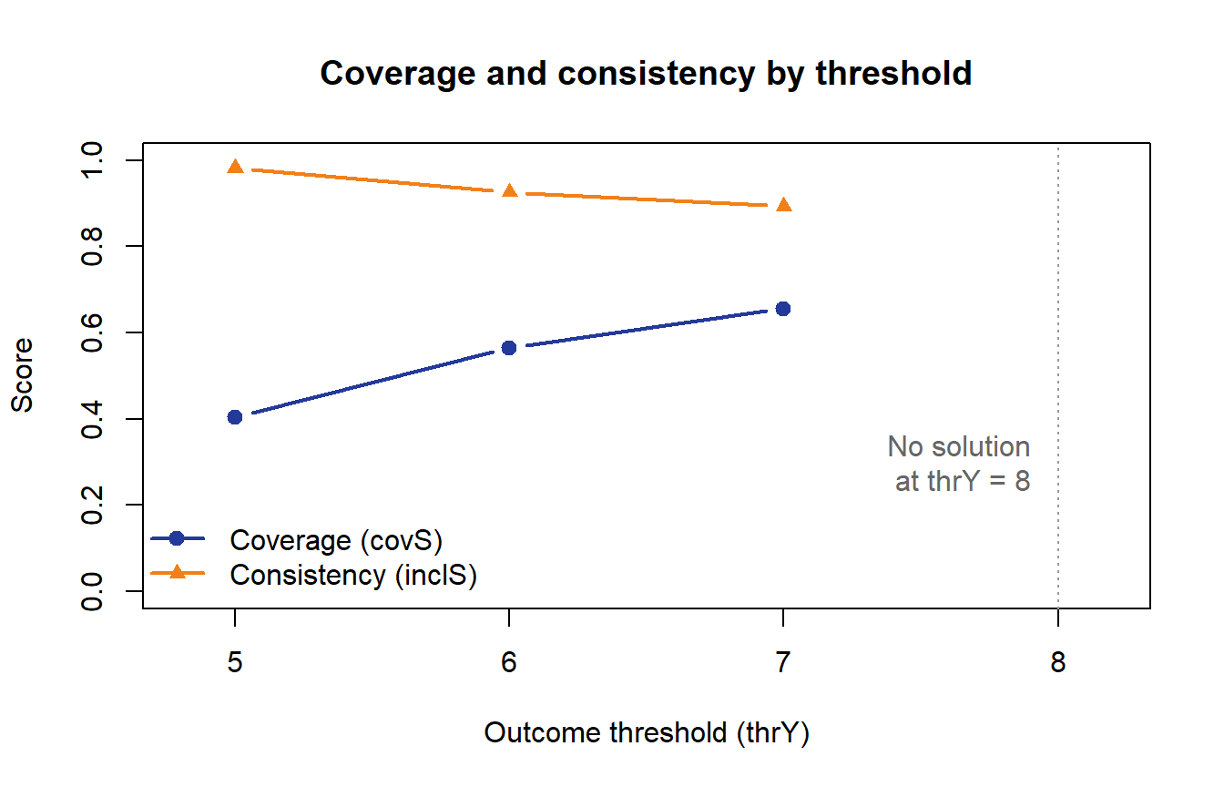

Solution coverage (covS) and solution consistency (inclS) at each outcome threshold. No solution was found at thrY = 8.

As the target gets higher, coverage rises (the solution explains a larger share of the high-loyalty customers) while consistency slowly falls. At thrY = 8 the line simply stops, because there is no solution to plot.

What comes next

In the next part we will look more closely at the four kinds of sweeps (outcome, one condition, several conditions, and both together), and at how to choose the range of thresholds in a way you can defend.

The full package tutorial is available in the ThSQCA documentation, and the methodology is described in Toyoda (2026), Quality & Quantity.

Software used: R 4.6.1, QCA 3.25.5, and ThSQCA 2.0.9.