library(ThSQCA)
library(QCA)
Loading required package: admisc
To cite package QCA in publications, please use:
  Dusa, Adrian (2019) QCA with R. A Comprehensive Resource.
Springer International Publishing.In the first three parts we ran sweeps and learned to read them. In this last part we turn a sweep into something you can report and defend: a written record of what was explored, a chart of the configurations, and a check that the numbers agree with the QCA package.
library(ThSQCA)
library(QCA)Loading required package: admisc
To cite package QCA in publications, please use:
Dusa, Adrian (2019) QCA with R. A Comprehensive Resource.
Springer International Publishing.make_demo_data <- function(n = 400, seed = 2026) {
set.seed(seed)
clip <- function(x) pmin(10, pmax(0, round(x)))
QUA <- clip(rnorm(n, 6, 2))
SER <- clip(rnorm(n, 6, 2))
ENV <- clip(rnorm(n, 6, 2))
core <- pmax(pmin(QUA, SER), pmin(QUA, ENV) - 1)
LOY <- clip(core + rnorm(n, 0, 0.7))
data.frame(LOY, QUA, SER, ENV)
}
demo <- make_demo_data()We reuse the outcome threshold sweep from part 1. This time we ask for the full details, which the report needs.
res_ots <- otSweep(
  dat            = demo,
  outcome        = "LOY",
  conditions     = c("QUA", "SER", "ENV"),
  sweep_range    = 5:8,
  thrX           = c(QUA = 7, SER = 7, ENV = 7),
  incl.cut       = 0.8,
  n.cut          = 1,
  return_details = TRUE
)
A sweep produces many results, and a reader needs to know what range was explored, under which settings, and what came out at each threshold. generate_report() writes this into a Markdown file. It comes in two formats.
"simple" is a short report for the main text or an appendix. It has a summary table, the solution at each threshold, and code for checking the result with the QCA package."full" is for supplementary material. It adds an overview of the analysis (the sweep range and the cutoffs), descriptive statistics, and, for every threshold, the truth table, the solution fit, per-term metrics, a configuration chart, the QCA package output, and the settings needed to reproduce it. A comparison across thresholds follows.report_file <- tempfile(fileext = ".md")
generate_report(res_ots, report_file, dat = demo, format = "simple")Here are the first lines of the file it wrote. On your own computer, give the file a real name, such as "ots_report_simple.md", and it will appear in your working folder.
cat(head(readLines(report_file), 25), sep = "\n")# QCA Analysis Report
*(Auto-generated by ThSQCA package)*
**Generated**: 2026-10-08 23:37
---
## Summary
| thrY | expression | inclS | covS | n_solutions |
|---|---|---|---|---|
| 5 | QUA\*SER + QUA\*ENV | 0.981 | 0.403 | 1 |
| 6 | QUA\*SER + QUA\*ENV | 0.926 | 0.565 | 1 |
| 7 | QUA\*SER | 0.894 | 0.656 | 1 |
| 8 | No solution | NA | NA | 0 |
---
## Solutions Overview
### LOY >= 5
**Solution**: QUA\*SER + QUA\*ENV -> LOYA few options are worth knowing:
generate_report(res_ots, "r.md", dat = demo, format = "full")              # more detail
generate_report(res_ots, "r.md", dat = demo, include_chart = FALSE)        # no charts
generate_report(res_ots, "r.md", dat = demo, chart_symbol_set = "latex")   # LaTeX symbols
generate_report(res_ots, "r.md", dat = demo, include_raw_output = FALSE) # omit QCA outputQCA papers often show solutions as a chart: one column per path, one row per condition, a filled circle for “present”, a crossed circle for “absent”, and a blank where the path does not restrict the condition (neither presence nor absence is required). You can draw one from a list of paths with config_chart_from_paths().
paths <- c("A*B*~C", "A*D", "B*E")
cat(config_chart_from_paths(paths))| Condition | T1 | T2 | T3 |
|---|---|---|---|
| A | ● | ● | |
| B | ● | ● | |
| C | ⊗ | ||
| D | ● | ||
| E | ● |
● = presence, ⊗ = absence, blank = don’t care
If you prefer plain characters, for example for a journal that cannot print the circle symbols, use the ASCII version:
cat(config_chart_from_paths(paths, symbol_set = "ascii"))| Condition | T1 | T2 | T3 |
|---|---|---|---|
| A | O | O | |
| B | O | O | |
| C | X | ||
| D | O | ||
| E | O |
O = presence, X = absence, blank = don’t care
A sweep table gives solutions and fit values, but not the number of cases behind them. A reader should be able to see that, because a result that rests on a handful of cases deserves less trust. For the outcome sweep of part 1, we can count the customers directly from the data, without ThSQCA.
thr <- 5:8
n_out  <- sapply(thr, function(t) sum(demo$LOY >= t))
n_both <- sapply(thr, function(t) sum(demo$LOY >= t & demo$QUA >= 7 & demo$SER >= 7))
cases <- rbind("High loyalty (LOY >= thrY)" = n_out,
               "... and high on QUA and SER" = n_both)
colnames(cases) <- thr

bp <- barplot(cases, beside = TRUE, col = c("#233A9A", "#F28018"),
              ylim = c(0, max(cases) * 1.15),
              xlab = "Outcome threshold (thrY)", ylab = "Number of customers",
              main = "Cases behind each threshold",
              legend.text = rownames(cases),
              args.legend = list(x = "topright", bty = "n", cex = 0.8))
text(bp, cases, labels = cases, pos = 3, cex = 0.8)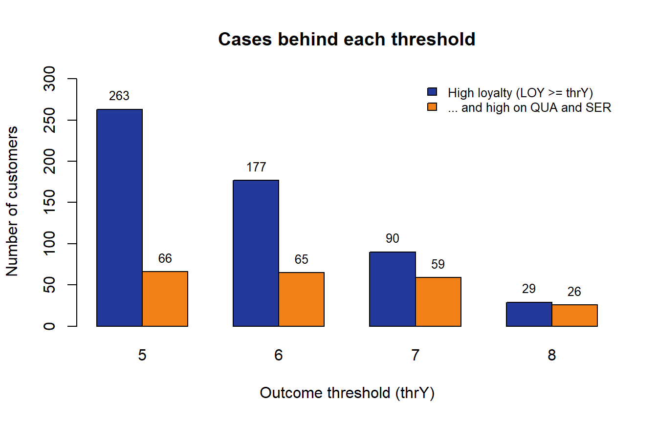
As the target rises, the high-loyalty group shrinks from 263 customers to 29, so the solutions at the strict end of a sweep are built on far fewer cases. Reporting these counts next to the sweep table is a simple way to show how much each row can bear.
ThSQCA does not invent new results. Every cell is an ordinary QCA analysis, so you can reproduce any cell by hand. This is a good way to build trust in the tool, and to answer a reviewer who asks. Here we reproduce the cell at an outcome threshold of 7.
bin <- function(x, t) as.integer(x >= t)

d7 <- data.frame(
  LOY = bin(demo$LOY, 7), QUA = bin(demo$QUA, 7),
  SER = bin(demo$SER, 7), ENV = bin(demo$ENV, 7)
)

tt  <- truthTable(d7, outcome = "LOY", conditions = c("QUA", "SER", "ENV"),
                  incl.cut = 0.8, n.cut = 1, show.cases = FALSE)
sol <- minimize(tt)
sol
M1: QUA*SER -> LOYThe solution printed by minimize() matches the row for thrY = 7 in the sweep table from part 1 (QUA*SER). In both cases the data were binarized in the same way (a score of 7 or above is a member), and in both cases the same QCA functions did the minimization.
Results can depend on the versions of R and the packages. Print them and keep them with your report:
c(R      = R.version.string,
  QCA    = as.character(packageVersion("QCA")),
ThSQCA = as.character(packageVersion("ThSQCA")))Because a sweep gives you freedom to explore, it also asks you to be transparent. Before you report one, make sure that you can answer yes to each of these questions.
You now know the whole workflow: choose a sweep, set a defensible range, run it, read it, and report it. If you want more, the package documentation has the full tutorial with additional examples, and the methodology is explained in the paper.
Software used: R 4.6.1, QCA 3.25.5, and ThSQCA 2.0.9.