library(ThSQCA)In part 1 we ran an outcome threshold sweep and read its result. ThSQCA has four sweep functions in total. This post runs all four on the same practice data, and ends with practical advice on choosing the range of thresholds.
The four sweeps at a glance
| Question | Function | What varies | What stays fixed |
|---|---|---|---|
| How does the solution change as the target level of the outcome rises? | otSweep() |
the outcome threshold | all condition thresholds |
| How sensitive is it to one condition’s definition of “high”? | ctSweepS() |
one condition threshold | the outcome and the other conditions |
| What if several conditions’ definitions change together? | ctSweepM() |
several condition thresholds (a grid) | the outcome threshold |
| What if the target level and the conditions’ definitions both change? | dtSweep() |
the outcome and the conditions | nothing |
Setup: the same practice data as part 1
Practice data (identical to part 1)
make_demo_data <- function(n = 400, seed = 2026) {
  set.seed(seed)
  clip <- function(x) pmin(10, pmax(0, round(x)))
  QUA <- clip(rnorm(n, 6, 2))
  SER <- clip(rnorm(n, 6, 2))
  ENV <- clip(rnorm(n, 6, 2))
  core <- pmax(pmin(QUA, SER), pmin(QUA, ENV) - 1)
  LOY  <- clip(core + rnorm(n, 0, 0.7))
  data.frame(LOY, QUA, SER, ENV)
}

demo <- make_demo_data()
Remember the story behind the data: loyalty (LOY) is high when quality (QUA) and service (SER) are both high, or, a little less strongly, when quality and the store environment (ENV) are both high.
Sweep 1: one condition with ctSweepS()
Suppose you are unsure where to draw the line for “high service delivery”. Is 6 high enough? 7? 9? Fix the outcome at LOY >= 7, fix the other conditions at 7, and sweep the threshold of SER from 5 to 9.
res_cts <- ctSweepS(
  dat          = demo,
  outcome      = "LOY",
  conditions   = c("QUA", "SER", "ENV"),
  sweep_var    = "SER",
  sweep_range  = 5:9,
  thrY         = 7,
  thrX_default = 7
)

summary(res_cts)
CTS (single) Summary
====================
Analysis Parameters:
Outcome: LOY
Conditions: QUA, SER, ENV
Consistency cutoff: 0.8
Frequency cutoff: 1
Results by Threshold:
threshold expression inclS covS n_solutions
5 No solution NA NA 0
6 No solution NA NA 0
7 QUA*SER 0.894 0.656 1
8 QUA*SER 0.909 0.333 1
9 QUA*SER*~ENV 0.917 0.122 1The new arguments are sweep_var (the condition whose threshold is swept), thrY (the fixed outcome threshold), and thrX_default (the fixed threshold for all other conditions).
Reading the table from top to bottom: when “high service” is defined as 5 or 6, there is no solution, because the definition is so loose that the group of “highly served” customers is no longer reliably loyal. At 7 and 8 the solution is QUA*SER. At 9 the solution gains a third element, QUA*SER*~ENV, and coverage falls sharply, from 0.656 at 7 to 0.122 at 9. You can see why by counting how many customers are behind the strictest definition:
sum(demo$QUA >= 7 & demo$SER >= 9) # customers high on both quality and service[1] 16sum(demo$QUA >= 7 & demo$SER >= 9 & demo$ENV < 7) # customers satisfying the solution QUA*SER*~ENV[1] 12Of the 400 customers, 16 are high on both quality and service, and only 12 of them also have a store-environment score below 7, which is what the solution QUA*SER*~ENV requires. The result there rests on very few cases. This is a useful habit: when a solution appears only at the edge of the grid, check how many cases are behind it.
Sweep 2: several conditions with ctSweepM()
Now let the thresholds of all three conditions vary at once: each of QUA, SER, and ENV is tried at 6, 7, and 8. That is 3 x 3 x 3 = 27 combinations. The outcome stays at LOY >= 7.
res_mcts <- ctSweepM(
  dat        = demo,
  outcome    = "LOY",
  conditions = c("QUA", "SER", "ENV"),
  sweep_list = list(QUA = 6:8, SER = 6:8, ENV = 6:8),
  thrY       = 7
)
The output has 27 rows. To keep it readable, show only the combinations that produced a solution:
tab <- res_mcts$summary
tab[tab$n_solutions > 0, ]
combo_id threshold expression inclS covS
5 5 QUA=7, SER=7, ENV=6 QUA*SER 0.8939394 0.6555556
6 6 QUA=8, SER=7, ENV=6 QUA*SER 0.9189189 0.3777778
8 8 QUA=7, SER=8, ENV=6 QUA*SER 0.9090909 0.3333333
9 9 QUA=8, SER=8, ENV=6 QUA*SER 0.9047619 0.2111111
12 12 QUA=8, SER=6, ENV=7 QUA*SER*~ENV 0.8000000 0.3111111
14 14 QUA=7, SER=7, ENV=7 QUA*SER 0.8939394 0.6555556
15 15 QUA=8, SER=7, ENV=7 QUA*SER*~ENV 1.0000000 0.3000000
17 17 QUA=7, SER=8, ENV=7 QUA*SER 0.9090909 0.3333333
18 18 QUA=8, SER=8, ENV=7 QUA*SER*~ENV 1.0000000 0.1888889
21 21 QUA=8, SER=6, ENV=8 QUA*ENV 0.8888889 0.1777778
23 23 QUA=7, SER=7, ENV=8 QUA*SER 0.8939394 0.6555556
24 24 QUA=8, SER=7, ENV=8 QUA*SER + QUA*ENV 0.9200000 0.5111111
26 26 QUA=7, SER=8, ENV=8 QUA*SER 0.9090909 0.3333333
27 27 QUA=8, SER=8, ENV=8 QUA*SER*~ENV + QUA*~SER*ENV 0.9393939 0.3444444
n_solutions
5 1
6 1
8 1
9 1
12 1
14 1
15 1
17 1
18 1
21 1
23 1
24 1
26 1
27 1Some patterns to look for:
- Fourteen of the 27 combinations have a solution. In every combination where “high quality” is defined as 6, there is no solution at all.
- With
QUAat 7 andSERat 7 or 8, the solution isQUA*SERno matter which threshold is used forENV. This is a stable region. - With
QUAat 8, the solution depends onENV(and onSER). WithENVat 6 it isQUA*SER(whenSERis 7 or 8). WithENVat 7 it isQUA*SER*~ENV. WithENVat 8 it varies, fromQUA*ENValone to two-path solutions such asQUA*SER + QUA*ENV. When “high quality” is defined strictly, the definition of the store environment starts to matter.
The grid shows both where a conclusion is robust and where it is fragile, which a single analysis cannot.
Sweep 3: the outcome and the conditions together with dtSweep()
The dual threshold sweep combines the two ideas: it varies the target level of the outcome and the conditions’ definitions at the same time. Here we use 3 outcome thresholds (6, 7, 8) and 8 condition combinations (QUA, SER, ENV each at 6 or 7), so 24 cells.
res_dts <- dtSweep(
  dat           = demo,
  outcome       = "LOY",
  conditions    = c("QUA", "SER", "ENV"),
  sweep_list_X  = list(QUA = 6:7, SER = 6:7, ENV = 6:7),
  sweep_range_Y = 6:8
)

res_dts$summary
combo_id thrY thrX expression inclS covS
1 1 6 QUA=6, SER=6, ENV=6 QUA*SER 0.8630137 0.7118644
2 1 7 QUA=6, SER=6, ENV=6 No solution NA NA
3 1 8 QUA=6, SER=6, ENV=6 No solution NA NA
4 2 6 QUA=7, SER=6, ENV=6 QUA*SER 0.9215686 0.5310734
5 2 7 QUA=7, SER=6, ENV=6 No solution NA NA
6 2 8 QUA=7, SER=6, ENV=6 No solution NA NA
7 3 6 QUA=6, SER=7, ENV=6 QUA*SER 0.8932039 0.5197740
8 3 7 QUA=6, SER=7, ENV=6 No solution NA NA
9 3 8 QUA=6, SER=7, ENV=6 No solution NA NA
10 4 6 QUA=7, SER=7, ENV=6 QUA*SER 0.9848485 0.3672316
11 4 7 QUA=7, SER=7, ENV=6 QUA*SER 0.8939394 0.6555556
12 4 8 QUA=7, SER=7, ENV=6 No solution NA NA
13 5 6 QUA=6, SER=6, ENV=7 QUA*SER 0.8630137 0.7118644
14 5 7 QUA=6, SER=6, ENV=7 No solution NA NA
15 5 8 QUA=6, SER=6, ENV=7 No solution NA NA
16 6 6 QUA=7, SER=6, ENV=7 QUA*SER + QUA*ENV 0.9076923 0.6666667
17 6 7 QUA=7, SER=6, ENV=7 No solution NA NA
18 6 8 QUA=7, SER=6, ENV=7 No solution NA NA
19 7 6 QUA=6, SER=7, ENV=7 QUA*SER 0.8932039 0.5197740
20 7 7 QUA=6, SER=7, ENV=7 No solution NA NA
21 7 8 QUA=6, SER=7, ENV=7 No solution NA NA
22 8 6 QUA=7, SER=7, ENV=7 QUA*SER + QUA*ENV 0.9259259 0.5649718
23 8 7 QUA=7, SER=7, ENV=7 QUA*SER 0.8939394 0.6555556
24 8 8 QUA=7, SER=7, ENV=7 No solution NA NA
n_solutions
1 1
2 0
3 0
4 1
5 0
6 0
7 1
8 0
9 0
10 1
11 1
12 0
13 1
14 0
15 0
16 1
17 0
18 0
19 1
20 0
21 0
22 1
23 1
24 0Reading it: at LOY >= 6, every one of the 8 condition definitions gives a solution, usually QUA*SER, and sometimes QUA*SER + QUA*ENV. At LOY >= 7, only two definitions still give a solution, the ones where QUA and SER are both at 7. At LOY >= 8, none do. In this data set, raising the target level is the strongest driver of change.
A picture makes the same point faster. The next chunk draws the solution coverage of all 24 cells as a heat map. Each row is one definition of the three conditions, each column is one outcome threshold, and “none” marks a cell with no solution.
s <- res_dts$summary
m <- tapply(s$covS, list(s$combo_id, s$thrY), function(x) x[1])
lab <- as.character(s$thrX[match(rownames(m), s$combo_id)])

op <- par(mar = c(4.5, 11, 3, 1))
image(x = seq_len(ncol(m)), y = seq_len(nrow(m)), z = t(m),
      col = colorRampPalette(c("#FFFFFF", "#233A9A"))(50), zlim = c(0, 1),
      xaxt = "n", yaxt = "n", xlab = "Outcome threshold (thrY)", ylab = "",
      main = "Solution coverage in the 24 cells")
axis(1, at = seq_len(ncol(m)), labels = colnames(m))
axis(2, at = seq_len(nrow(m)), labels = lab, las = 1, cex.axis = 0.8)
for (i in seq_len(nrow(m))) for (j in seq_len(ncol(m))) {
  if (is.na(m[i, j])) text(j, i, "none", col = "grey50", cex = 0.8)
  else text(j, i, sprintf("%.2f", m[i, j]), cex = 0.8)
}
box()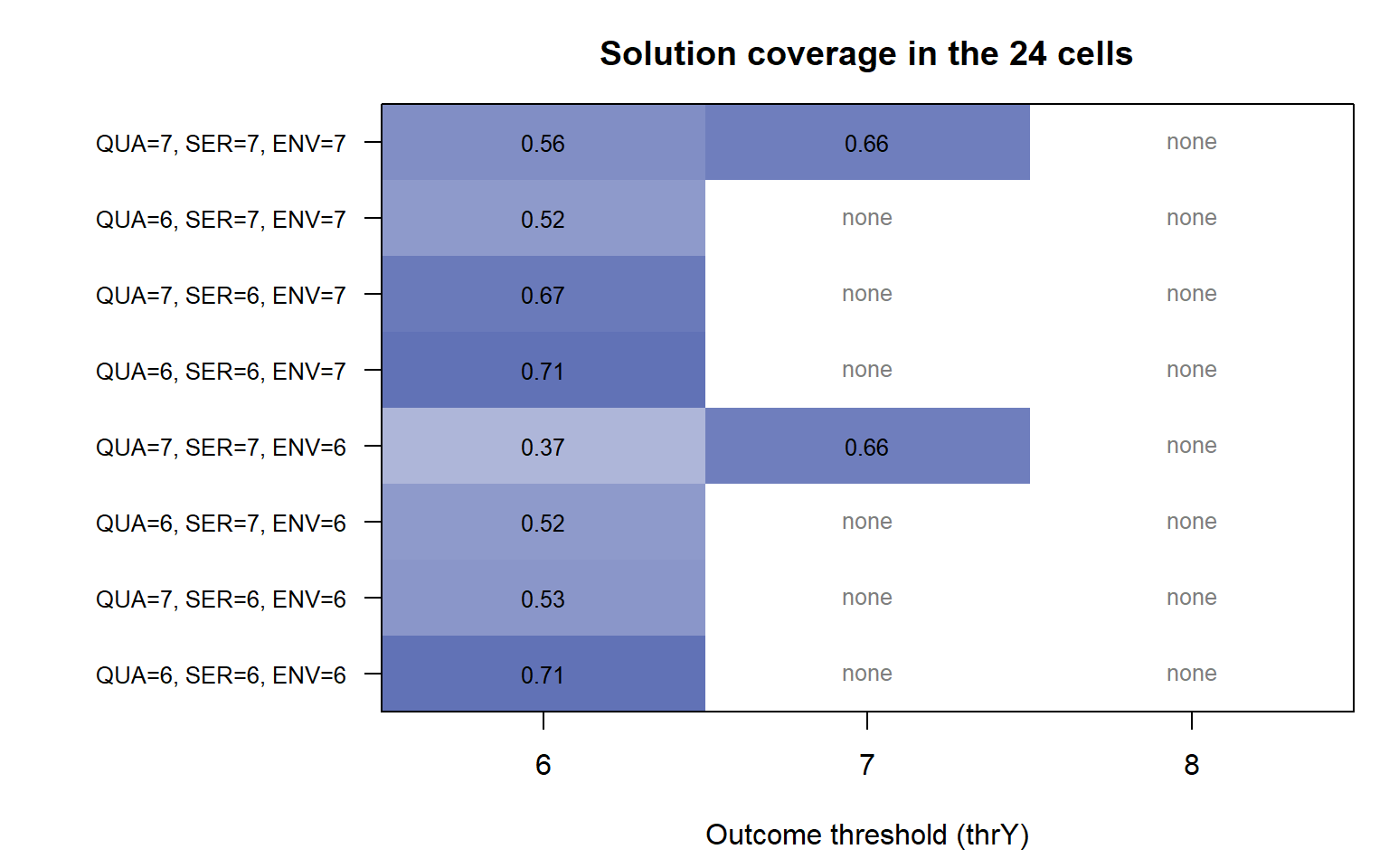
par(op)The column for LOY >= 6 is filled in every row, the column for LOY >= 7 in only two, and the column for LOY >= 8 in none.
How big is a sweep?
Every cell is a full QCA analysis, so the number of cells matters for run time and for how readable the results are.
| Function | Number of analyses | Example |
|---|---|---|
otSweep() |
one per outcome threshold | 5 thresholds = 5 |
ctSweepS() |
one per threshold of the swept condition | 5 thresholds = 5 |
ctSweepM() |
the product of the candidate counts | 3 x 3 x 3 = 27 |
dtSweep() |
outcome thresholds x condition grid | 3 x (3 x 3 x 3) = 81 |
Choosing a range you can defend
A sweep is easy to run, which is exactly why it needs discipline. Trying many thresholds and reporting only the convenient ones would add researcher degrees of freedom instead of removing them. Some rules of thumb:
- Decide the range before you look at the results. Base it on what the scale means, on theory, and on practical targets (for example “acceptable”, “good”, “very good”).
- Include your baseline. The threshold you would have used in an ordinary analysis should be inside the grid, so readers can compare.
- Avoid the neutral zone. On a 0 to 10 scale, scores around the midpoint do not clearly mean “high” for anyone, so ranges usually start above it.
- Keep the grid small enough to read. A few meaningful values per variable are better than every possible value.
- Check the case counts at the edges. Cells at the extremes of the grid often rest on very few cases.
- Report the whole grid. Show the stable and the unstable regions, not only the cells that support your story.
What comes next
In part 3 we look at the three solution types (complex, parsimonious, and intermediate) and at what to do when a cell has more than one minimal solution.
Software used: R 4.6.1, QCA 3.25.5, and ThSQCA 2.0.9.